Tioga Pass Opening Date
Every winter, Tioga Pass in Yosemite National Park closes due to the snow and the unsafe driving conditions. Depending on the snowfall for the year and the road conditions, Tioga Pass opens between May and June. Tioga Pass usually opens to bikes only for a week, and then it opens to the general public afterwards. What’s a reasonable prediction for the 2021 Tioga Pass Opening Date?
Cleaning the Data
First, let’s import the historical opening dates from the NPS. The National Park Service (NPS) has recorded the historical opening dates for Tioga Pass since the 1980s.
import pandas as pd
import numpy as np

df = pd.read_csv('.../yose-Websitesortabledataelementsheetsroadscampgroundstrails.csv')
df
| Year | Tioga Opened | Tioga Closed | Glacier Pt Opened | Glacier Pt Closed | Mariposa Grove Opened | Mariposa Grove Closed | Snowpack as of Apr 1 | |
|---|---|---|---|---|---|---|---|---|
| 0 | 2020 * | 15-Jun | 5-Nov | 11-Jun | 5-Nov | 11-Jun | 25-Dec | 46% |
| 1 | 2019 * | 1-Jul | 19-Nov | 10-May | 25-Nov | 16-Apr | 26-Nov | 176% |
| 2 | 2018 * | 21-May | 20-Nov | 28-Apr | 20-Nov | 15-Jun | 30-Nov | 67% |
| 3 | 2017 * | 29-Jun | 14-Nov | 11-May | 14-Nov | Closed | Closed | 177% |
| 4 | 2016 * | 18-May | 16-Nov | 19-Apr | 16-Nov | Closed | Closed | 89% |
| 5 | 2015 * | 4-May | 1-Nov | 28-Mar | 2-Nov | No closure | 6-Jul | 7% |
| 6 | 2014 * | 2-May | 13-Nov | 14-Apr | 28-Nov | No closure | No closure | 33% |
| 7 | 2013 | 11-May | 18-Nov | 3-May | 18-Nov | No closure | No closure | 52% |
| 8 | 2012 | 7-May | 8-Nov | 20-Apr | 8-Nov | No closure | No closure | 43% |
| 9 | 2011 * | 18-Jun | 17-Jan | 27-May | 19-Nov | 15-Apr | No closure | 178% |
| 10 | 2010 | 5-Jun | 19-Nov | 29-May | 7-Nov | 21-May | 20-Nov | 107% |
| 11 | 2009 | 19-May | 12-Nov | 5-May | 12-Nov | NaN | NaN | 92% |
| 12 | 2008 | 21-May | 30-Oct | 2-May | 12-Dec | NaN | NaN | 99% |
| 13 | 2007 | 11-May | 6-Dec | 4-May | 6-Dec | NaN | NaN | 46% |
| 14 | 2006 | 17-Jun | 27-Nov | 25-May | 27-Nov | NaN | NaN | 129% |
| 15 | 2005 | 24-Jun | 25-Nov | 25-May | ? | NaN | NaN | 163% |
| 16 | 2004 | 14-May | 17-Oct | 14-May | ? | NaN | NaN | 83% |
| 17 | 2003 | 31-May | 31-Oct | 31-May | 31-Oct | NaN | NaN | 65% |
| 18 | 2002 | 22-May | 5-Nov | 17-May | 5-Nov | NaN | NaN | 95% |
| 19 | 2001 | 12-May | 11-Nov | 15-May | ? | NaN | NaN | 67% |
| 20 | 2000 | 18-May | 9-Nov | 15-May | 9-Nov | NaN | NaN | 97% |
| 21 | 1999 * | 28-May | 23-Nov | 28-May | 23-Nov | NaN | NaN | 110% |
| 22 | 1998 | 1-Jul | 12-Nov | 1-Jul | 6-Nov | NaN | NaN | 156% |
| 23 | 1997 | 13-Jun | 12-Nov | 22-May | 12-Nov | NaN | NaN | 105% |
| 24 | 1996 | 31-May | 5-Nov | 24-May | 5-Nov | NaN | NaN | 111% |
| 25 | 1995 | 30-Jun | 11-Dec | 1-Jul | 11-Dec | NaN | NaN | 178% |
| 26 | 1994 | 25-May | 10-Nov | NaN | NaN | NaN | NaN | 51% |
| 27 | 1993 | 3-Jun | 24-Nov | NaN | NaN | NaN | NaN | 159% |
| 28 | 1992 | 15-May | 10-Nov | NaN | NaN | NaN | NaN | 58% |
| 29 | 1991 | 26-May | 14-Nov | NaN | NaN | NaN | NaN | 79% |
| 30 | 1990 | 17-May | 19-Nov | NaN | NaN | NaN | NaN | 45% |
| 31 | 1989 | 12-May | 24-Nov | NaN | NaN | NaN | NaN | 83% |
| 32 | 1988 | 29-Apr | 14-Nov | NaN | NaN | NaN | NaN | 31% |
| 33 | 1987 | 2-May | 13-Nov | NaN | NaN | NaN | NaN | 51% |
| 34 | 1986 | 24-May | 29-Nov | NaN | NaN | NaN | NaN | 137% |
| 35 | 1985 | 8-May | 12-Nov | NaN | NaN | NaN | NaN | 97% |
| 36 | 1984 | 19-May | 8-Nov | NaN | NaN | NaN | NaN | 85% |
| 37 | 1983 | 29-Jun | 11-Nov | NaN | NaN | NaN | NaN | 224% |
| 38 | 1982 | 28-May | 15-Nov | NaN | NaN | NaN | NaN | 131% |
| 39 | 1981 | 15-May | 12-Nov | NaN | NaN | NaN | NaN | 77% |
| 40 | 1980 | 6-Jun | 2-Dec | NaN | NaN | NaN | NaN | 144% |
| 41 | Average\n('96-'15) | 26-May | 14-Nov | 14-May | 15-Nov | -- | -- | 92% |
| 42 | Median\n('96-'15) | 21-May | 12-Nov | 16-May | 10-Nov | -- | -- | 96% |
The only columns needed for analysis are “Year” and “Tioga Opened,” and the other columns can be dropped.
Using April 1st as a reference date, I created the function formatDates() to calculate the number of days since April 1st that Tioga Pass opened for each year, appending to the new column “Days Since Apr 1.”
import datetime

df = df.drop([41, 42])
df = df.drop(columns=['Tioga Closed', 'Glacier Pt Opened', 'Glacier Pt Closed', 'Mariposa Grove Opened', 'Mariposa Grove Closed', 'Snowpack as of Apr 1'])
df['Days Since Apr 1'] = 0

def formatDates(row):
    snowpack_day = datetime.datetime.strptime('1900-04-01 00:00:00', '%Y-%m-%d %H:%M:%S')
    tioga_open = datetime.datetime.strptime(row, '%d-%b')
    days_since = tioga_open - snowpack_day
    return days_since.days

for i in range(len(df)):
    df.iloc[i, 2] = formatDates(df.iloc[i, 1])

df
| Year | Tioga Opened | Days Since Apr 1 | |
|---|---|---|---|
| 0 | 2020 * | 15-Jun | 75 |
| 1 | 2019 * | 1-Jul | 91 |
| 2 | 2018 * | 21-May | 50 |
| 3 | 2017 * | 29-Jun | 89 |
| 4 | 2016 * | 18-May | 47 |
| 5 | 2015 * | 4-May | 33 |
| 6 | 2014 * | 2-May | 31 |
| 7 | 2013 | 11-May | 40 |
| 8 | 2012 | 7-May | 36 |
| 9 | 2011 * | 18-Jun | 78 |
| 10 | 2010 | 5-Jun | 65 |
| 11 | 2009 | 19-May | 48 |
| 12 | 2008 | 21-May | 50 |
| 13 | 2007 | 11-May | 40 |
| 14 | 2006 | 17-Jun | 77 |
| 15 | 2005 | 24-Jun | 84 |
| 16 | 2004 | 14-May | 43 |
| 17 | 2003 | 31-May | 60 |
| 18 | 2002 | 22-May | 51 |
| 19 | 2001 | 12-May | 41 |
| 20 | 2000 | 18-May | 47 |
| 21 | 1999 * | 28-May | 57 |
| 22 | 1998 | 1-Jul | 91 |
| 23 | 1997 | 13-Jun | 73 |
| 24 | 1996 | 31-May | 60 |
| 25 | 1995 | 30-Jun | 90 |
| 26 | 1994 | 25-May | 54 |
| 27 | 1993 | 3-Jun | 63 |
| 28 | 1992 | 15-May | 44 |
| 29 | 1991 | 26-May | 55 |
| 30 | 1990 | 17-May | 46 |
| 31 | 1989 | 12-May | 41 |
| 32 | 1988 | 29-Apr | 28 |
| 33 | 1987 | 2-May | 31 |
| 34 | 1986 | 24-May | 53 |
| 35 | 1985 | 8-May | 37 |
| 36 | 1984 | 19-May | 48 |
| 37 | 1983 | 29-Jun | 89 |
| 38 | 1982 | 28-May | 57 |
| 39 | 1981 | 15-May | 44 |
| 40 | 1980 | 6-Jun | 66 |
The snow depth data dates back to 2005, so the Tioga Pass opening dates can be reduced to 2005-2020.
# Drops the years before 2005, and reverses the dataframe so data is sorted from old --> new.
df = df[0:16]
df = df[::-1].reset_index(drop=True)
df
| Year | Tioga Opened | Days Since Apr 1 | |
|---|---|---|---|
| 0 | 2005 | 24-Jun | 84 |
| 1 | 2006 | 17-Jun | 77 |
| 2 | 2007 | 11-May | 40 |
| 3 | 2008 | 21-May | 50 |
| 4 | 2009 | 19-May | 48 |
| 5 | 2010 | 5-Jun | 65 |
| 6 | 2011 * | 18-Jun | 78 |
| 7 | 2012 | 7-May | 36 |
| 8 | 2013 | 11-May | 40 |
| 9 | 2014 * | 2-May | 31 |
| 10 | 2015 * | 4-May | 33 |
| 11 | 2016 * | 18-May | 47 |
| 12 | 2017 * | 29-Jun | 89 |
| 13 | 2018 * | 21-May | 50 |
| 14 | 2019 * | 1-Jul | 91 |
| 15 | 2020 * | 15-Jun | 75 |
Next, let’s import the snow depth data from the California Data Exchange Center. The station of interest is in Tuolumne Meadows (TUM).
import pandas as pd
df_TUM = pd.read_excel('.../TUM_18.xlsx')
df_TUM
| STATION_ID | DURATION | SENSOR_NUMBER | SENS_TYPE | DATE TIME | OBS DATE | VALUE | DATA_FLAG | UNITS | |
|---|---|---|---|---|---|---|---|---|---|
| 0 | TUM | D | 18 | SNOW DP | NaN | 20041001.0 | 2.0 | INCHES | |
| 1 | TUM | D | 18 | SNOW DP | NaN | 20041002.0 | 0.0 | INCHES | |
| 2 | TUM | D | 18 | SNOW DP | NaN | 20041003.0 | -0.0 | INCHES | |
| 3 | TUM | D | 18 | SNOW DP | NaN | 20041004.0 | 0.0 | INCHES | |
| 4 | TUM | D | 18 | SNOW DP | NaN | 20041005.0 | 1.0 | INCHES | |
| ... | ... | ... | ... | ... | ... | ... | ... | ... | ... |
| 6004 | TUM | D | 18 | SNOW DP | NaN | 20210310.0 | 38.0 | INCHES | |
| 6005 | TUM | D | 18 | SNOW DP | NaN | 20210311.0 | 118.0 | INCHES | |
| 6006 | TUM | D | 18 | SNOW DP | NaN | 20210312.0 | 118.0 | INCHES | |
| 6007 | TUM | D | 18 | SNOW DP | NaN | 20210313.0 | 42.0 | INCHES | |
| 6008 | TUM | D | 18 | SNOW DP | NaN | 20210314.0 | NaN | INCHES |
6009 rows × 9 columns
The only columns needed for analysis are “OBS DATE” and “VALUE.” “DATE TIME” can also be kept, since we’ll need to convert the OBS DATE into a datetime object.
Other columns can be dropped, and any rows with missing snow data can also be dropped.
# Drops the columns that are no longer needed.
# Drops rows with NaN values in the VALUE or OBS DATE columns
df_TUM = df_TUM.drop(columns=['STATION_ID', 'DURATION', 'SENSOR_NUMBER', 'SENS_TYPE', 'DATA_FLAG', 'UNITS'])
df_TUM = df_TUM.dropna(subset=['VALUE']).reset_index(drop=True)
df_TUM = df_TUM.dropna(subset=['OBS DATE']).reset_index(drop=True)
df_TUM
| DATE TIME | OBS DATE | VALUE | |
|---|---|---|---|
| 0 | NaN | 20041001.0 | 2.0 |
| 1 | NaN | 20041002.0 | 0.0 |
| 2 | NaN | 20041003.0 | -0.0 |
| 3 | NaN | 20041004.0 | 0.0 |
| 4 | NaN | 20041005.0 | 1.0 |
| ... | ... | ... | ... |
| 5432 | NaN | 20210309.0 | 36.0 |
| 5433 | NaN | 20210310.0 | 38.0 |
| 5434 | NaN | 20210311.0 | 118.0 |
| 5435 | NaN | 20210312.0 | 118.0 |
| 5436 | NaN | 20210313.0 | 42.0 |
5437 rows × 3 columns
# Convert the OBS DATE column to string format
df_TUM['OBS DATE'] = df_TUM['OBS DATE'].astype(int)
df_TUM['OBS DATE'] = df_TUM['OBS DATE'].astype(str)

# Adds on the DATE TIME column by converting the string form of OBS DATE to pandas TimeStamp object
df_TUM['DATE TIME'] = pd.to_datetime(df_TUM['OBS DATE'], format='%Y%m%d')
df_TUM
| DATE TIME | OBS DATE | VALUE | |
|---|---|---|---|
| 0 | 2004-10-01 | 20041001 | 2.0 |
| 1 | 2004-10-02 | 20041002 | 0.0 |
| 2 | 2004-10-03 | 20041003 | -0.0 |
| 3 | 2004-10-04 | 20041004 | 0.0 |
| 4 | 2004-10-05 | 20041005 | 1.0 |
| ... | ... | ... | ... |
| 5432 | 2021-03-09 | 20210309 | 36.0 |
| 5433 | 2021-03-10 | 20210310 | 38.0 |
| 5434 | 2021-03-11 | 20210311 | 118.0 |
| 5435 | 2021-03-12 | 20210312 | 118.0 |
| 5436 | 2021-03-13 | 20210313 | 42.0 |
5437 rows × 3 columns
With the daily snow depth data from 2004-2020, let’s average the snow depth data for each month.
# Groupby the month and year
TUM_avg = df_TUM.groupby([(df_TUM['DATE TIME'].dt.year),(df_TUM['DATE TIME'].dt.month)]).mean()
TUM_avg
| VALUE | ||
|---|---|---|
| DATE TIME | DATE TIME | |
| 2004 | 10 | 9.833333 |
| 11 | 22.166667 | |
| 12 | 35.258065 | |
| 2005 | 1 | 78.064516 |
| 2 | 78.250000 | |
| ... | ... | ... |
| 2020 | 11 | 15.033333 |
| 12 | 24.258065 | |
| 2021 | 1 | 33.838710 |
| 2 | 50.642857 | |
| 3 | 50.538462 |
196 rows × 1 columns
Once the snow depth data has been averaged, let’s group the data by month. For example, the TUM_1 dataframe will include the average snow depth for each January from 2005-2020.
# Set the name of the multiindex
TUM_avg.index.names = ['Year', 'Month']

# Select January subset from the multiindex dataframe
TUM_1 = TUM_avg[TUM_avg.index.get_level_values('Month') == 1]
TUM_1
| VALUE | ||
|---|---|---|
| Year | Month | |
| 2005 | 1 | 78.064516 |
| 2006 | 1 | 70.058824 |
| 2007 | 1 | 20.483871 |
| 2008 | 1 | 54.870968 |
| 2009 | 1 | 27.774194 |
| 2010 | 1 | 44.800000 |
| 2011 | 1 | 66.428571 |
| 2012 | 1 | 8.178571 |
| 2013 | 1 | 54.407407 |
| 2014 | 1 | 4.933333 |
| 2015 | 1 | 8.866667 |
| 2016 | 1 | 51.137931 |
| 2017 | 1 | 73.782609 |
| 2018 | 1 | 24.483871 |
| 2019 | 1 | 49.580645 |
| 2020 | 1 | 29.129032 |
| 2021 | 1 | 33.838710 |
# Repeat for all 12 months
TUM_2 = TUM_avg[TUM_avg.index.get_level_values('Month') == 2]
TUM_3 = TUM_avg[TUM_avg.index.get_level_values('Month') == 3]
TUM_4 = TUM_avg[TUM_avg.index.get_level_values('Month') == 4]
TUM_5 = TUM_avg[TUM_avg.index.get_level_values('Month') == 5]
TUM_6 = TUM_avg[TUM_avg.index.get_level_values('Month') == 6]
TUM_7 = TUM_avg[TUM_avg.index.get_level_values('Month') == 7]
TUM_11 = TUM_avg[TUM_avg.index.get_level_values('Month') == 11]
TUM_12 = TUM_avg[TUM_avg.index.get_level_values('Month') == 12]
Given that the snow depth data has been averaged for each of the 12 months spanning 2005-2020, we can create a subset of the TUM_3 dataframe that excludes 2021 data.
TUM_3_Historical = TUM_3[TUM_3.index.get_level_values('Year') != 2021]
TUM_3_Historical
| VALUE | ||
|---|---|---|
| Year | Month | |
| 2005 | 3 | 81.548387 |
| 2006 | 3 | 89.200000 |
| 2007 | 3 | 31.225806 |
| 2008 | 3 | 55.645161 |
| 2009 | 3 | 58.387097 |
| 2010 | 3 | 66.548387 |
| 2011 | 3 | 83.333333 |
| 2012 | 3 | 20.793103 |
| 2013 | 3 | 37.000000 |
| 2014 | 3 | 19.724138 |
| 2015 | 3 | 1.064516 |
| 2016 | 3 | 44.566667 |
| 2017 | 3 | 97.516129 |
| 2018 | 3 | 50.709677 |
| 2019 | 3 | 93.870968 |
| 2020 | 3 | 34.709677 |
Plotting the Data
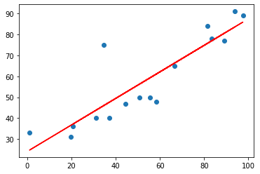
Now that the data has been processed, it’s time to plot the data and build the model. A simple linear regression between Days Since April 1st and Snow Depth in March can be performed.
import matplotlib.pyplot as plt
from sklearn.linear_model import LinearRegression

x = TUM_3_Historical['VALUE'].values.reshape(-1, 1)
y = df['Days Since Apr 1'].values.reshape(-1, 1)

linear_regressor = LinearRegression()  # Create object for the class
linear_regressor.fit(x, y)  # Perform linear regression
y_pred = linear_regressor.predict(x)  # Make predictions

plt.plot(x, y_pred, color='red')
plt.scatter(x, y)
plt.show()
from scipy.stats import linregress
slope, intercept, r_value, p_value, std_err = linregress(x.flatten().tolist(), y.flatten().tolist())
results = linregress(x.flatten().tolist(), y.flatten().tolist())
print(results)
print('R-squared:', r_value**2)
LinregressResult(slope=0.6338435941606729, intercept=24.074433161488514, rvalue=0.8816178208666444, pvalue=6.354407547787794e-06, stderr=0.09068732698031783, intercept_stderr=5.541187818860552)
R-squared: 0.7772499820696507
The scatterplot shows a moderately strong, positive, linear association between Days Since April 1st and Snow Depth in March, with one potential outlier. 77.7% of the variability in Days Since April 1st is accounted by the LSR model on Snow Depth in March.
With the LRS model, we can approximate the number of Days Since April 1st that Tioga Pass will open this year based on the Snow Depth data for March 2021.
current_snow_depth = TUM_3['VALUE'].iloc[-1]
print(current_snow_depth, 'inches')

predicted_days = slope*current_snow_depth + intercept
print(np.round(predicted_days), 'days since April 1')
50.53846153846154 inches
56.0 days since April 1
raw_date = datetime.date(2021, 4, 1) + datetime.timedelta(np.round(predicted_days))
print(raw_date)
2021-05-27
Historically, NPS has always opened Tioga Pass on a Monday. As such, May 27 needs to be rounded to the following Monday.
import datetime
def nextMonday(date):
    monday = 0
    days_ahead = monday - date.weekday() + 7
    return date + datetime.timedelta(days_ahead)

predicted_date = nextMonday(raw_date)
print(predicted_date)
2021-05-31
Conclusion
Based on the snow depth data up to March 13, 2021, my prediction for this year’s Tioga Pass Opening Date is May 31, 2021.